


Most Data 360 cost overruns I have seen came from processes nobody was watching: an identity resolution ruleset re-evaluating profiles all day, a handful of unmonitored Calculated Insights refreshing every hour, or a build team iterating on full production volume because nobody told them not to.
Data 360 is a consumption-based platform, so each of those processes draws down credits regardless of whether anyone is looking. The hard part is knowing where to spend your governance effort for maximum impact on your cost profile.
The answer is building a credit feedback loop: a small set of architectural choices and queries that make Data 360 credit consumption visible both while you are building and once you are live.
Test build logic against a filtered data set
The build phase is where you iterate the most and, by default, where you pay the most for work you are about to throw away. Every time you remap a field, rerun unification, rebuild a Calculated Insight, or test a segment on full volume, you spend a part of the production credits to validate logic. At this stage, it is important to test your logic, but there is no need to test it against large amounts of data.
A good strategy here is to prevent the build from running on production-scale data. Before ingestion, apply filters at the data space level on every object that feeds unification, typically Contacts and Accounts, so the entire downstream pipeline, mapping through identity resolution, Calculated Insights, segmentation, and activation, operates on a small but representative slice.
By applying filters, you can validate the model and the outputs against a slice of data, and then walk the client through the results. After the client confirms the logic, you remove the filters and migrate the build to production.
Filtering the build keeps its cost to a small fraction of the contract. Across more than four different project implementations that I recently worked on, the entire build and test phase stayed under 5% of the client’s total purchased credit allotment. On a 10,000 credit entitlement, that is under 500 credits for the full build and test cycle, leaving the rest for production, which is where those credits deliver their primary business value.
Two conditions decide whether this works for you. First, the sample has to be representative: choose records that exercise your real identity overlaps and data quality problems, not the first few thousand rows, or your identity resolution testing will lie to you. Second, anything that does depend on volume behavior, such as activation performance at scale, has to be tested deliberately and separately, rather than by leaving the filters off for the whole engagement.
Keeping the filter at the data space level, rather than scattering it across streams or data transforms, is important, because it stays consistent across every object and lifts in one place at cutover.




Know which processes draw down credits
Once you are live, the biggest credit costs often come from automated background work, not from the features you deliberately built. Processes like identity resolution and scheduled Calculated Insights keep running and drawing credits long after launch.
Identity resolution is the easiest one to underestimate. On any day, if X new records are ingested, the total number of records processed by identity resolution is almost always higher than X. This is because, in addition to processing new records, it also re-evaluates some of the existing profiles that are impacted by the new profiles, and credits are consumed based on the number of processed records, not the number of records ingested. In addition, changing a ruleset, a match rule, or a reconciliation rule triggers a full reprocessing of every source profile, which can dwarf a day’s ingestion and is easy to miss because no new data arrived. You can make projections at design time by referring to the rate card, but treat them as hypotheses: estimate during design, then validate against actual consumption once you are live, because the real volume rarely matches the projections written on a design diagram.
Calculated Insights consume credits in the same way. Their cost is the volume processed multiplied by how often they refresh, so a single insight left on an hourly schedule costs twenty-four times what it would cost if refreshed daily. Transforms, queries, and activations add their own draw, because each traverses the Data Model Objects (DMOs) on its path and processes every record it crosses.
The takeaway is to set each insight’s refresh cadence to how often its inputs actually change, not to a default. To gauge that, look at how often the source data updates and how often the downstream consumer, such as a segment, an activation, or an agent action, actually reads the value.
Again, you can estimate these costs at design time from projections, but a projection is only a hypothesis until the platform proves it right or wrong. You validate it by measuring actual consumption, which is where instrumentation comes in, and where an estimate that was off by an order of magnitude becomes visible before the invoice does.
Measure consumption with Digital Wallet, then trace the spike
Start where the platform already helps you. Digital Wallet Consumption Cards give you a high-level understanding at a glance. For each card, it shows what you purchased, what you have consumed, and what remains.
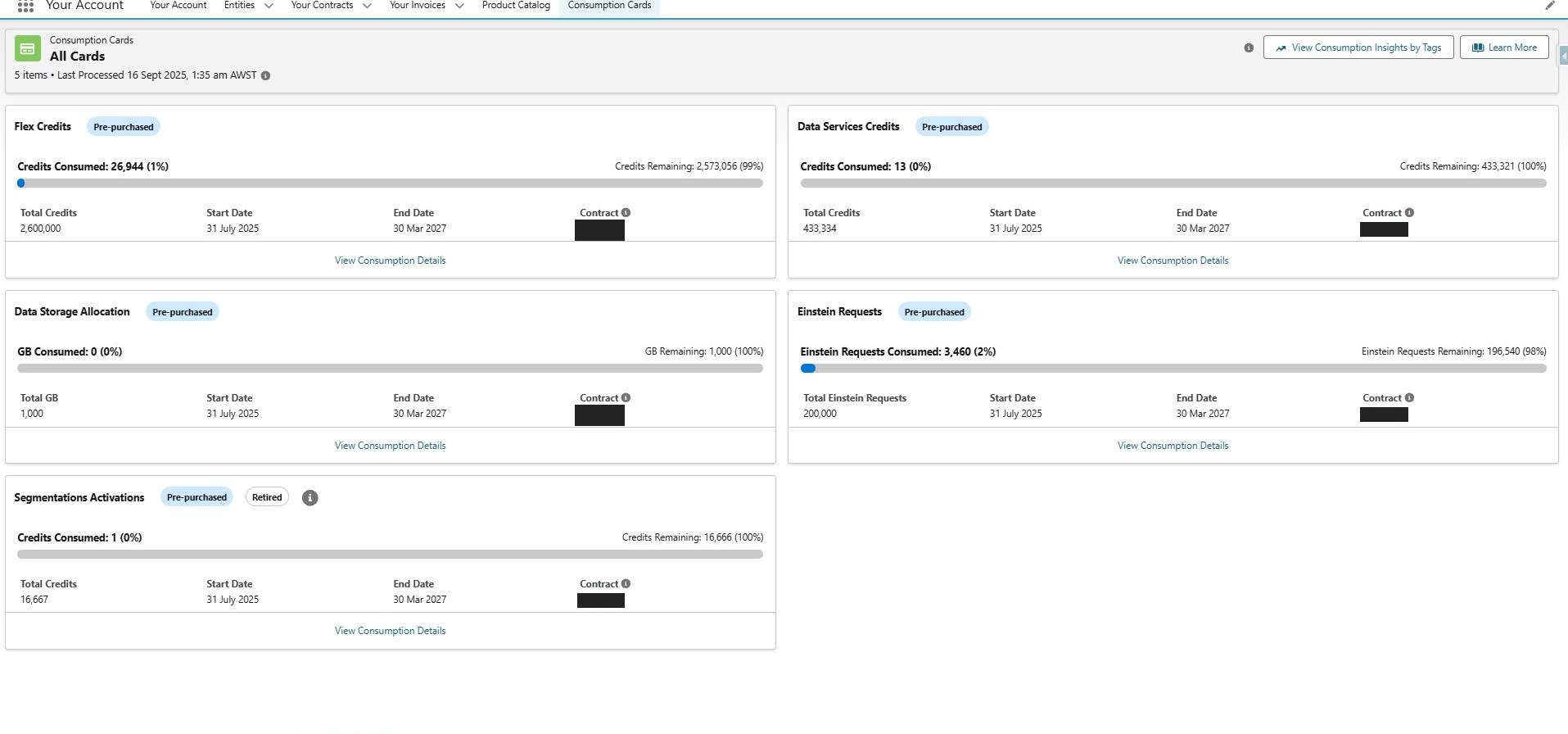
This answers the two key questions right away. Is any card burning faster than its share of the contract term? Which usage type dominates your spend? For routine health checks, you can stop here.
When you open a card, the platform goes a level deeper. The Consumption Insights page plots consumption per day, so the single most expensive day is obvious without writing a line of SQL, and the Consumption By Type table breaks down that spend by environment, usage type, and multiplier.
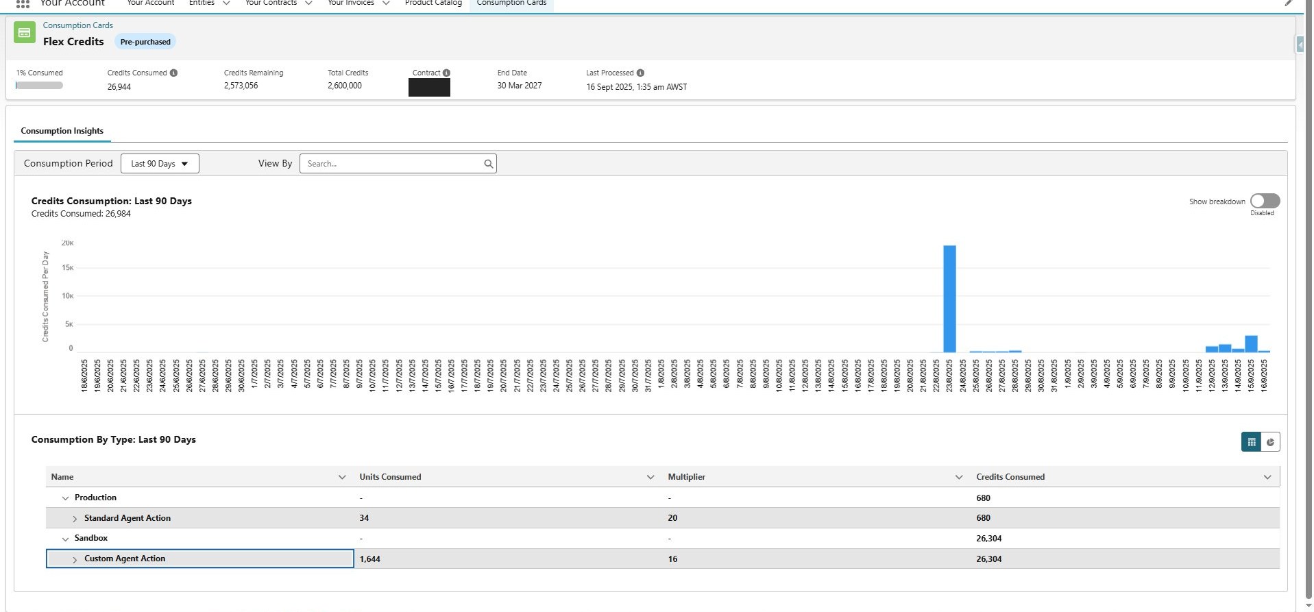
That is about as far as the built-in views go. They give you the what, the when, and the broad type. What they do not give you is which specific resource ran, in which hour, for how long, or whether one operation or a recurring schedule produced the spike. For those answers, you query four Data Lake Objects (DLOs) that sit beneath the cards.
Dive deeper into consumption by querying the DLOs
Each object answers a different question. TenantDailyEntitlementConsumption and TenantHourlyEntitlementConsumption hold the credit math, raw usage, unit, multiplier, and the resulting credits, at daily and hourly grain. TenantBillingUsageEvent holds the individual events with precise timestamps. TenantEntitlementTransaction holds what was purchased.
Add the ones you need to your data space to make them queryable. Map each to a DMO if you want to create a report on them, since the standard Salesforce platform reporting tools look at the DMO layer rather than at raw DLOs.
A few specifics can help make these run easily. Data 360 SQL addresses a DLO as ObjectName__dll, and date and timestamp literals need a cast. The credit-bearing field in both consumption objects is unitsconsumed__c; usageconsumed__c is the raw, unweighted usage, and unit__c and multiplier__c are what convert one into the other.
The hourly object must be filtered to rowdetail__c = 'PROCESSED', because it also holds in-flight rows that would otherwise inflate your totals. Both consumption objects also carry an environment field, usagebusinessenvtype__c on the daily object and businessenvtype__c on the hourly and billing objects, indispensable when you want to separate production from sandbox.
Start by surfacing only the days worth investigating. Finding the single most expensive day is something the cards already do, so instead compute each card’s own 30-day average and return the days that ran well above it:
WITH daily AS (
  SELECT CAST(utilizationdate__c AS date) AS usage_day,
         carddefinitiondevelopername__c   AS card,
         SUM(unitsconsumed__c)            AS credits
  FROM   TenantDailyEntitlementConsumption__dll
  WHERE  utilizationdate__c >= CURRENT_DATE - INTERVAL '30' day
  GROUP  BY CAST(utilizationdate__c AS date), carddefinitiondevelopername__c
),
scored AS (
  SELECT usage_day, card, credits,
         AVG(credits) OVER (PARTITION BY card) AS avg_per_day
  FROM   daily
)
SELECT usage_day, card, credits, avg_per_day
FROM   scored
WHERE  credits > avg_per_day * 1.5
ORDER  BY credits - avg_per_day DESC;
Each row is a card and a day that broke its own pattern, judged against that card’s normal rather than one global number. On a quiet month, the query returns nothing, which is exactly what you want a monitor to say.
For a flagged day, for example the late-August spike above, find what consumed the credits. The hourly object carries resource attribution and the credit total together, so you can rank actual credits by resource and by hour:
SELECT usagehourbucket__c,
       resourcetype__c,
       resourceidorapiname__c,
       SUM(unitsconsumed__c) AS credits_consumed
FROM   TenantHourlyEntitlementConsumption__dll
WHERE  usagehourbucket__c >= CAST('2025-08-23 00:00:00' AS timestamp)
  AND  usagehourbucket__c <  CAST('2025-08-24 00:00:00' AS timestamp)
  AND  rowdetail__c = 'PROCESSED'
GROUP  BY usagehourbucket__c, resourcetype__c, resourceidorapiname__c
ORDER  BY credits_consumed DESC
LIMIT  20;
This names the resource and the hour. Usage in a single hour points to a one-off job; usage in every hour points to a schedule, which is how you catch a Calculated Insight set to refresh more often than anyone needs.
When you need the precise window, drop to the event level. TenantBillingUsageEvent timestamps every event, and links the events of one logical operation through CorrelationIdentifier__c, so you can measure how long an operation actually ran using the following query:
SELECT CorrelationIdentifier__c,
	 RootResourceType__c,
       RootResourceidOrApiName__c,
       MIN(EventTime__c)  AS first_event,
       MAX(EventTime__c)  AS last_event,
       EXTRACT(EPOCH FROM (MAX(EventTime__c) - MIN(EventTime__c))) / 60
                          AS duration_minutes,
       COUNT(*)           AS event_count
FROM   TenantBillingUsageEvent__dll
WHERE  EventTime__c >= CAST('2025-08-23 00:00:00' AS timestamp)
  AND  EventTime__c <  CAST('2025-08-24 00:00:00' AS timestamp)
GROUP  BY CorrelationIdentifier__c, RootResourceType__c, RootResourceidOrApiName__c
ORDER  BY duration_minutes DESC
LIMIT  20;
None of this is on the consumption graphs. The cards tell you a spike happened and its broad type; the DLOs take you further: which resource ran, in which hour, and for how long, and, because the daily and hourly objects carry raw usage, the unit, and the multiplier side by side (usageconsumed__c, unit__c, and multiplier__c), whether volume or a multiplier drove the cost. And because TenantEntitlementTransaction records what you purchased as quantity__c per card, you can measure consumption against your remaining runway.
One warning: these queries read raw usage data and draw query credits themselves. For routine reporting rather than one-off investigation, use the TenantEnrichedUsageEvent DLO, which Salesforce built and optimized for consumption reporting: you can report on it directly without incurring query credits. Once you can attribute consumption this precisely, governance becomes a data problem you can alert on instead of a monthly surprise.
Data 360 SQL Reference
The dialect reference behind the queries above. Use it when you adapt the date filters or build your own aggregations, so the syntax matches the Data 360 query engine rather than a generic SQL dialect.



Use these recommendations to tune based on what you measure
Measurement only pays off when you act on it, and the highest-return action I have found is matching refresh cadence to how often a decision actually changes.
On a recent Agentforce build for a professional services business, enabling prompt template tracking caused Data 360 to auto-create five Calculated Insights: Prompt Template Feedback, Prompt Template Feedback Reasons, Prompt Template Generation Count, Prompt Template Version Feedback, and Prompt Template Version Feedback Reasons.
All five were set to refresh hourly. We wanted the adoption data, but nobody was reading it hourly, so the schedule was paying for freshness that no one used. Moving the five to a daily refresh cut their refresh cost to a twenty-fourth of what hourly refreshing cost, with no loss of value.
Schedule is a crucial lever, but not the only one Salesforce documents for Calculated Insights. Giving an insight to a start and end date stops it running once its purpose has passed, so any insight that only needs to run for a defined period should carry an end date rather than running open-ended.
Where you do not need point-in-time snapshots, turning off Track History removes the data queries that maintaining that history would otherwise consume. Salesforce billing considerations for Calculated Insights set out all three options together.
The cadence rule generalizes beyond Calculated Insights. Every scheduled process in Data 360 (a data transform, a segment refresh, or an activation) runs on a cadence someone chose once and rarely revisits. Match each cadence to how often the downstream decision actually changes, not to whatever default the platform sets, and the savings compound across the estate.
Make visibility part of the architecture
Data 360 will only process more data as agentic workloads expand, and every new agent, insight, and activation adds another process that draws credits in the background. The teams that stay in control will be the ones who build credit visibility into the architecture.
Pick one process you cannot currently attribute, write the query that puts a number on it, and decide this week whether that number is one you meant to spend.
Discover tips and resources created for architects, by architects
Explore Salesforce architecture thought leadership, insights, and best practices to build healthy solutions.