


It has been empirically observed
that different local optima, obtained from training deep neural networks
don’t generalize in the same way for the unseen data sets, even if they
achieve the same training loss. Recently, this problem has received
renewed interest from both the empirical and theoretical deep learning
communities. From the theoretical standpoint, most of the generalization
bounds developed for explaining this phenomenon only consider a worst-case
scenario, thus ignoring the generalization capabilities among different
solutions. In this blog we are interested in the following question:
We discuss several related proposals and introduce our recent work that
builds a connection between the model generalization and the Hessian of
the loss function.
img.animated-gif {
width: 450px;
height: auto;
}
.column {
float: left;
width: 33.33%;
padding: 5px;
}
.row::after {
content: “”;
clear: both;
display: table;
}
Empirical Observations on Hessian and Generalization
Hochreiter
and Schmidhuber, and more recently, Chaudhari et. al. and Keskar et al. argue that the
local curvature, or “sharpness”, of the converged solutions for deep
networks is closely related to the generalization property of the
resulting classifier. The sharp minimizers, which led to lack of
generalization ability, are characterized by a significant number of large
positive eigenvalues in (nabla^2 hat{L}(x)), the loss function being
minimized.
Neyshabur et al.
point out the sharpness itself may not be enough to determine the
generalization capability. They argue that it is necessary to include
the scales of the solution with sharpness to be able to explain
generalization. To this end, they suggest an “expected sharpness” based
on the PAC-Bayes bound: $$E_{usim N(0,sigma^2)^m}[hat{L}(w+u)] –
hat{L}(w)$$
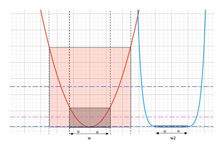
As shown in the figure below, intuitively if the local minima is
“smooth” then perturbing the model won’t cause the objective to change
much. Thus it provides a way of measuring the smoothness of the local
minima.

How to Perturb the Model?
It is well known that adding noise
to the model during training can help improving the model generalization.
However, how to set proper noise levels remains unknown. Most
state-of-the-art methods assume same level of perturbation along all
directions, but intuition suggests that this may not be appropriate.
Let’s look at a toy example. We construct a small 2-dimensional sample set
from a mixture of (3) Gaussians, and binarize the labels by thresholding
them from the median value. Then we use a (5)-layer MLP model with only
two parameters (w_1) and (w_2) for prediction, and the cross entropy
as the loss. The variables from different layers are shared. Sigmoid is
used as the activation function. The loss landscape of a model trained
using (100) samples is plotted below:
If we look at the optima indicated by the orange vertical bar, the
smoothness of the loss surface along different directions is quite
different. Should we impose the same level of perturbations along all
directions? Perhaps not.
We argue that more noise should be put along the “flat” directions.
Specifically, we suggest adding uniform or (truncated) Gaussian noise
whose level, in each coordinate direction, is roughly proportional to
$$sigma_i approx frac{1}{sqrt{nabla^2_{i,i} hat{L}+ rho N_{gamma,
epsilon}(w_i)} },$$ where (rho) is the local Lipschitz constant of the
Hessian (nabla^2hat{L}), and (N_{gamma, epsilon}(w_i)=gamma |w_i|
+ epsilon).
A Metric on Model Generalization
As discussed by Dinh et al. and Neyshabur et al., the spectrum of
Hessian itself may not be enough to determine the generalization power of a
model. In particular, for a multi-layer perceptron with RELU as the activation
function, one may re-parameterize the model and scale the Hessian spectrum
arbitrarily without affecting the model prediction and generalization.
Employing some approximations, we propose a metric on model generalization,
called PACGen, that depends on the scales of the parameters, the Hessian, and
the high-order smoothness terms that are characterized by the Lipschitz contant
of Hessian.
$$Psi_{gamma, epsilon}(hat{L}, w^ast) = sum_i log
left((|w_i^ast| + N_{gamma,epsilon}(w_i^ast))maxleft(sqrt{nabla^2_i
hat{L}(w^ast) + rho(w^ast)sqrt{m}N_{gamma,epsilon}(w_i^ast)},
frac{1}{N_{gamma,epsilon}(w_i^ast)}right)right),$$ where we assume
(hat{L}(w)) is locally convex around (w^ast).
Even though we
assume the local convexity in our metric, in application we may calculate the
metric on any point on the loss surface. When (nabla^2_i hat{L}(w^ast) +
rho(w^ast)sqrt{m}N_{gamma,epsilon}(w_i^ast) < 0), we simply treat it as
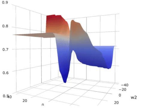
(0 ). The metric is plotted as the color wrapped on the surface in the figure
below.
Landscape of the loss on
a (2)-parameter (5) layer MLP with shared parameters. The colors over the
loss surface indicate the metric of generalization. Lower metric score indicates
better potential generalization power. The colors on the bottom plane indicate
an approximate generalization bound considering both the loss and the
generalization metric.
As displayed in the figure, the metric score around the global optimum,
indicated by the green vertical bar, is high, suggesting possible poor
generalization capability as compared to the local optimum indicated by the red
bar.
On the other hand, the overall expected loss is determined by
both the loss and the metric. For that we plotted a color plane on the bottom
of the figure. The color on the projected plane indicates an approximated
generalization bound, which considers both the loss and the generalization
metric. The local optimum indicated by the red bar, though has a slightly
higher loss, has a similar overall bound compared to the “sharp” global
optimum.
Reconstruction from the Model
Assuming the model is generating
(y=f(x)=p(y|x)), since we know the true distribution (p(x)), we can
reconstruct the join distribution (p(x,y)=p(x)p(y|x)). To be specific, we
first sample (x) from (p(x)), then use the model to predict
(hat{y}=f(x)). The samples sampled from the true distribution, the
distribution induced by the “sharp” minima and the “flat” minima, are shown
below.
Samples sampled from
the true distribution.
Predicted labels from
the “sharp” minima.
Predicted labels from
the “flat” minima.
The prediction function from the “flat” minima seems to have a simpler dicision
boundary as compared that of the “sharp” minima, even though the “sharp” minima
fits the labels better.
When PAC-Bayes meets Hessian Lipschitz
In order to get
a quantative evaluation of the local optimum and the model perturbation, we
need to look at the PAC-Bayes bound:
[PAC-Bayes-Hoeffding
Bound] Let (l(f, x,y)in [0,1]), and (pi) be any fixed distribution
over the parameters (mathcal{W}). For any (delta>0) and (eta>0),
with probability at least (1-delta) over the draw of (n) samples, for
any (w) and any random perturbation (u), $$mathbb{E}_u [L(w+u)]leq
mathbb{E}_u [hat{L}(w+u)] + frac{KL(w+u||pi) + log
frac{1}{delta}}{eta} + frac{eta}{2n}$$
Suppose (hat{L}(w^ast)) is the loss function at a local optima
(w^ast), when the perturbation level of (u) is small,
(mathbb{E}_u[hat{L}(w^ast+u)]) tends to be small, but
(KL(w^ast+u|pi)) may be large since the posterior is too focused on a
small neighboring area around (w^ast), and vice versa. As a consequence,
we may need to search for an optimal perturbation level for (u) so that
the bound is minimized.
For that we need some assumptions on the smoothness of the Hessian:
[Hessian Lipschitz] A twice differentiable function
(f(cdot)) is (rho)-Hessian Lipschitz if:
$$forall w_1, w_2, |nabla^2 f(w_1) – nabla^2 f(w_2)|leq rho
|w_1-w_2|,$$
where (|cdot|) is the operator norm.
Suppose the empirical loss function (hat{L}(w)) satisfies the
Hessian Lipschitz condition in some local neighborhood (Neigh_{gamma,
epsilon}(w)), then the perturbation of the function around a fixed
point can be bounded by terms up to the third-order,
(Nesterov) $$hat{L}(w+u) leq hat{L}(w) + nabla hat{L}(w)^T u +
frac{1}{2}u^T nabla^2 hat{L}(w) u + frac{1}{6}rho|u|^3~~~~forall
u~~s.t.~~ w+uin Neigh_{gamma,epsilon}(w)$$
Combine the PAC-Bayes bound and we get $$mathbb{E}_u [L(w+u)]leq hat{L}(w)
+frac{1}{2} sum_i nabla_{i,i}^2 hat{L}(w)mathbb{E} [u_i^2] +
frac{rho}{6}mathbb{E}[|u|^3] + frac{KL(w+u||pi) + log
frac{1}{delta}}{eta} + frac{eta}{2n}$$
Pluging in different perturbation distributions we can explicitly calculate the
KL divergence and solve for the best level of perturbation for each parameter.
PACGen on Real Data Sets
The PACGen metric is calculated on a PyTorch
model with various batch size and learning rate. We had similar
observations as Keskar et al. that as the batch size grows, the gap between
the test loss and the training loss tends to get larger. Our proposed metric
(Psi_{gamma, epsilon}(hat{L}, w^ast)) also shows the exact same
trend.


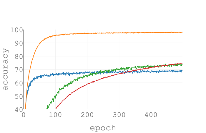
(Psi_{gamma=0.1, epsilon=0.1}) as a function of epochs on MNIST for
different batch sizes. SGD is used as the optimizer, and the learning rate
is set as (0.1) for all configurations. As the batch size grows,
(Psi_{gamma, epsilon}(hat{L}, w^ast)) gets larger. The trend is
consistent with the true gap of losses.


(Psi_{gamma=0.1, epsilon=0.1}) as a function of epochs on CIFAR10 for
different batch sizes. SGD is used as the optimizer, and the learning rate
is set as (0.01) for all configurations.
Similarly if we fix the training batch size as (256), as the learning rate
decreases, the gap between the test loss and the training loss increases, which
is also consistent with the trend calculated from (Psi_{gamma,
epsilon}(hat{L}, w^ast)).


(Psi_{gamma=0.1, epsilon=0.1}) as a function of epochs on MNIST for
different learning rates. SGD is used as the optimizer, and the batch size
is set as (256) for all configurations. As the learning rate shrinks,
(Psi_{gamma, epsilon}(hat{L}, w^ast)) gets larger. The trend is
consistent with the true gap of losses.


(Psi_{gamma=0.1, epsilon=0.1}) as a function of epochs on CIFAR10 for
different learning rates. SGD is used as the optimizer, and the batch size
is set as (256) for all configurations.
Pertubed Optimization
PAC-Bayes bound suggests we should optimize the perturbed loss instead of the true loss for a better generalization. In particular, the level of perturbation on each parameter is set according to the local smoothness property. We observe improved performance for the perturbed model on CIFAR-10, CIFAR-100, as well as the tiny Imagenet data sets.


Conclusion and Citation Credit
We connect the smoothness of the solution with the model generalization in the PAC-Bayes framework. We theoretically show that the generalization power of a model is related to the Hessian and the smoothness of the solution, the scales of the parameters, as well as the number of training samples. Based on our generalization bound, we propose a new metric to test the model generalization and a new perturbation algorithm that adjusts the perturbation levels according to the Hessian. Finally, we empirically demonstrate the effect of our algorithm is similar to a regularizer in its ability to attain better performance on unseen data. For more details, including details regarding the proof and its assumptions, please refer to our pre-print.
Identifying Generalization Properties in Neural Networks Huan Wang, Nitish Shirish Keskar, Caiming Xiong and Richard Socher.